Batch TD(0) as Dynamic Programming on the Empirical MRP
Motivation
This post grew out of Chapter 6 of Sutton and Barto's Reinforcement
Learning: An Introduction. In their discussion of batch updating, they
note that batch TD(0) converges to the certainty-equivalence estimate. This
was not obvious to me at the time, and I found it very interesting because it
shows how TD uses the Markov structure of the environment through the Bellman
equation, which is important for understanding why, in some cases, TD methods
can be more sample-efficient than methods like Monte Carlo.
The book does not explain this relationship in much detail, so I thought it
would be a good learning exercise to derive it myself. Since the goal of the
post was learning, I worked through the derivations with pen and paper. After
that, I took photos of the pages and used Codex / GPT 5.4 to help check the
derivations and overall logic, translate them into HTML, and write the code
for the experiment and visualizations.
Problem Statement & Approach
Let us consider a prediction problem rather than a control problem. We want to evaluate the state-value function of a fixed policy $\pi(a \mid s)$ from a finite collection of observed trajectories. The same general logic can later be extended to state-action value functions, but here I focus only on state values.
In this section I will show that if batch TD(0) is run until convergence, then its fixed point coincides with the fixed point obtained by the following two-stage procedure:
estimate the policy-induced Markov Reward Process from the observed trajectories by maximum likelihood;
run dynamic programming policy evaluation on that estimated model.
Let us now formalize the assumptions and the claim.
Claim
We assume a finite episodic Markov Reward Process induced by a fixed policy $\pi$, and a collection of trajectories sampled from that same process. A single trajectory is
Markov reward process. The policy-induced process satisfies the Markov property:
$$P(S_{t+1}, R_{t+1} \mid S_t, S_{t-1}, R_t, \dots) = P(S_{t+1}, R_{t+1} \mid S_t).$$
Time-homogeneous dynamics. The policy-induced transition-reward law does not depend on time:
$$P(S_{t+k+1}, R_{t+k+1} \mid S_{t+k}) = P(S_{t+1}, R_{t+1} \mid S_t).$$
Reward-model restriction. For each observed transition pair $(s, s')$, we restrict attention to conditional reward models $p_\pi(r \mid s, s')$ whose maximum-likelihood estimator has conditional expectation equal to the empirical mean reward over all observed transitions from $s$ to $s'$.
Under these assumptions, the fixed point of the Bellman operator
where $N(s)$ is the number of times state $s$ was visited across all trajectories.
Before going further, let us define the following notation:
$S$: the set of all observed nonterminal states,
$S^+$: the set of all observed states, including terminal states.
Proof Plan
When I was deriving these results, I intuitively followed steps:
Derive the fixed-point equation of batch TD(0)
Rewrite the Bellman fixed-point equation for the policy-induced process into a form that makes its connection to the batch TD(0) fixed point explicit
Compute the maximum-likelihood estimators of the relevant transition and reward probability distributions from the observed trajectories, substitute them into the reformulated Bellman equation, and verify that the resulting fixed point is exactly the same as the fixed point of batch TD(0).
In practice I iterated between the first two steps several times, but this is the cleanest way to present the argument.
Here we average over all trajectories and all time steps within each trajectory for which we observed state $s$.
However, there is an additional simplification, notice that the term $S_{t+1}$ represents the state visited immediately after $s$. It is easy to notice that the update to a state value function $v(s)$ is bootstrapped only from states that followed state $s$ across all observed trajectories. This can be expressed using a simple indicator function:
Notice that when we sum over all timestamps, we don't enforce sum over set $[t: S_t = s]$, and the reason for that is the intersection of states where $S_t=s$ and $S_t=s \land S_{t+1}=s'$ is $S_t=s \land S_{t+1}=s'$, so with the indicator function we added, we can sum over all $t$.
If you look at the inner sum it is just number of times across all trajectories where state $s$ was followed by state $s'$, which is exactly $N(s, s')$
Now all we are left with is outer sum
Summing over all successor states $s' \in S^+$, the bootstrapped value part becomes
$$
\gamma \sum_{s' \in S^+} N(s,s') v(s').
$$
Part 3: current-state value term
Finally, consider the term involving $v(s)$. Since $v(s)$ does not depend on $s', i, or \ t$, it can be factored out of all sums
Notice, that we already saw two inner sums, in Part 2 of the derivation and they are just equal to $N(s, s')$, now $\sum_{s' \in S^+} N(s, s') = N(s)$, which is just number of times we saw state $s$ in all of the trajectories.
Part 4: Putting the three parts together
Substituting the three simplified expressions back into the fixed-point equation, we obtain
We only evaluate this equation for states $s \in S$, so $N(s)>0$. Also, $\bar r(s,s')$ is only defined for observed transition pairs with $N(s,s')>0$, pairs with $N(s,s')=0$ contribute zero in the indicator-based form.
Fixed Point of MLE + DP
Let us split this part into two subsections. In the first, we simplify the Bellman operator; in the second, we compute the necessary maximum-likelihood estimates from existing trajectories and express the Bellman operator through those estimates.
Simplify Bellman Operator
Given the Bellman operator of the policy-induced Markov Reward Process
Now after we rewrote Bellman operator we see the probabilities that we need to find maximum likelihood for $p_{\pi}(s'|s)$ and $p_{\pi}(r| s', s)$. And it is intuitively clear at this point if you look at fixed point of TD(0) what MLE of these distributions should be.
Maximum Likelihood Estimation
Maximum likelihood of trajectory
Even though from this point onward we work directly with the policy-induced MRP, it is useful to
make explicit how the MRP trajectory law is derived from the underlying MDP under a fixed policy.
Consider first the MDP view of a single trajectory:
such that the probability of observed trajectories is maximized, i.e. we parameterize both distributions and find parameters such that likelihood of observing trajectories we see is maximized.
MLE for Transition Kernel $p_{\pi}(s' | s)$
Claim
Assuming a direct categorical parameterization of the transition kernel, with no additional structural assumptions, i.e. $p_{\pi}(s'|s) = \theta_{\pi,s,s'}$ and $\sum_{s'}\theta_{\pi,s,s'} = 1$
Note, if a single transition probability is categorical, because we can have multiple it translates into a multinomial, and we get that in order to find $\theta$ that maximizes likelihood of trajectory, we need
On the other hand, after rewriting the Bellman operator under the policy-induced probability measure, we showed that policy evaluation in the induced MRP can be written as
Therefore, the equivalence with MLE + DP holds only when the $p^{MLE}_{\pi}(r | s, s')$ is such that the conditional expectation of reward
coincides with this empirical conditional mean. This is true for many common models (Gaussian), but not for all (e.g. Laplace).
Substituting these two estimators into the Bellman operator gives
But this is exactly the same equation as the fixed-point equation of batch TD(0). Therefore, the fixed point of batch TD(0) coincides with the fixed point obtained by
estimating the policy-induced transition and reward model by maximum likelihood from the observed trajectories, and then
running dynamic programming policy evaluation with that estimated model.
In other words, batch TD(0) converges to the state-value function that is the fixed point of the Bellman equation for the empirical MRP induced by the maximum-likelihood model estimated from the data. If you view it this way, TD(0) is not just an update rule - it is implicitly solving that Bellman fixed-point equation by leveraging the Markov structure of the problem.
Experiment: What approach is better and when?
In the previous part of the blog, we derived that the fixed point of empirical model + DP is the same as the fixed point of batch TD(0). In this part, I want to understand which regimes are better suited for each approach. For a second, let's think about the time complexity. A single batch TD sweep over all trajectories is linear in the total number of sampled transitions; if we denote that number by $m$, then one batch TD sweep costs $O(m)$.
For certainty-equivalent evaluation, we first compile the sampled transitions into an empirical MRP. This construction scans the $m$ sampled transitions once, but the resulting model stores only the $E$ unique observed transition edges, where an edge is a distinct state-transition tuple $(s,s')$ with $N(s,s') > 0$. After that, one application of the empirical Bellman operator costs $O(E)$. Instead of repeatedly applying the Bellman operator, one could also solve the linear DP problem directly, for example by solving $(I - \gamma \hat P)v = \hat r$. A naive matrix inverse would be unstable and would ignore sparsity, so in the experiments below I use repeated applications of the empirical Bellman operator until convergence as the baseline DP solver.
Radius Knob: Increasing Empirical Branching
Intuitively, it is clear that the larger the number of edges is, the more advantageous it becomes to use TD(0). So the main idea of the experiment is to have an environment where we can experiment with different levels of connectivity between states. We start from a very sparse version of the environment and gradually move to a denser one.
The environment is very simple: you start from the upper-left point on a $256 \times 256$ grid and need to get to the goal point in the lower-right corner. The fixed policy is deterministic: it moves right until it reaches the last column, and then moves down toward the goal. With probability $0.75$, the environment respects this choice. With probability $0.25$, it teleports you. The knob that regulates teleportation is what moves the environment from sparse connections between states to dense connections between states. The visualization below is a miniature version of the same geometry.
Current stateGoalPolicy moveTeleport candidates
15 teleport candidates
Teleport probability0.25
Experiment states65536
Local probability0.75
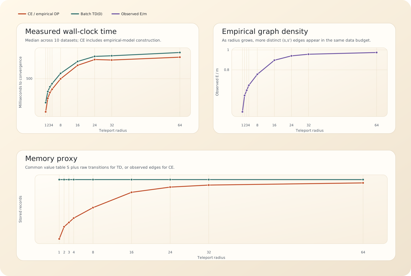
For different values of teleportation radius, I collect exactly 6K sampled transitions. Then I run two approaches (batch TD(0) and Empirical MRP + DP) to the same convergence tolerance.
One interesting aspect here is that in the experiment I set $\alpha = 1$, which algebraically makes both updates equivalent. For a state $s$, the batch TD update becomes
So in this experiment the two methods perform the same mathematical update. They just use different representations: batch TD operates on raw sampled transitions, while the certainty-equivalent version operates on the compressed set of observed edges, and as such will almost always be faster at the sweep stage. The problem is that building that compressed representation, the empirical MRP, is costly, despite being done only once.
The efficiency of this compression depends on how many times the same edge was visited. If many raw samples repeat the same transition $(s,s')$, then the empirical MRP can replace all of those repeated samples with one edge count and one average reward. But the smaller the number of repeated visits per edge, the less compression the empirical MRP provides. In the limiting case where every observed edge is visited only once, Empirical MRP + DP gives no compression gain during the update stage, but still pays the upfront cost of constructing the edge representation.
To compare empirical behavior, the left plot reports wall-clock time for this Python implementation. For each radius, I generate 10 independent datasets and plot the median runtime. The Empirical MRP + DP timing includes building the empirical model from the 6K transitions and then applying the empirical Bellman operator until convergence. The batch TD timing includes preparing the raw transition representation and then sweeping over those transitions until convergence.
These timings are implementation-dependent, but they answer the practical question directly: in this implementation, which approach finishes faster as the environment becomes more connected? The graph-density plot shows the reason for the trend by tracking $E/m$, the fraction of raw samples that remain as unique observed edges. The memory plot uses stored records as a simple proxy: batch TD stores roughly $S + m$ values/transitions, while Empirical MRP + DP stores roughly $S + E$ values/edges.
Results are generated from 10 independent simulated datasets per radius; wall-clock values are medians from the local Python implementation.
As we mentioned, batch TD touches $m$ raw transitions each sweep, while Empirical MRP + DP touches $E$ empirical edges after the model has been built. As the radius grows, $E/m$ rises, and the compressed empirical model becomes less cheap relative to replaying the batch.