RL for LLMs, Part I: From REINFORCE to the Policy Gradient Theorem - Derive Everything Yourself

Deriving policy gradients through exercises

When I was studying different areas of mathematics, my favorite thing was to try proving results myself, step by step, before reading their proofs. Doing this forced me to confront details I would otherwise have missed while reading a textbook, and often led to new insights. It also felt weirdly satisfying, like you really accomplished something! This post is an attempt to compile from different sources a set of intermediate results that allows me and reader to derive everything from first principles.

Of course, I couldn't always prove a result in one go and so I would usually try to find a staircase of lemmas / smaller results, each giving me something I needed for the next step, until the final "aha" moment of getting to the result. The steps had to be manageable enough that I could make progress, but challenging enough to keep me engaged and allow me to learn (tbh, after writing this I thought that this specific complexity requirement sounds very much similar to task complexity you would want in RL methods)

In this post, step by step, we will get to two points:

1. Derive REINFORCE and its several variants.
2. Connect the REINFORCE derivation to the policy gradient theorem.

The goal is to rederive each result yourself. I will split the derivation into small directed graph of results: you can prove them, open a hint, or read the worked solutions. Gradually you will derive most of the results necessary for understanding policy gradient methods. The only prerequisites for this post are probably Chapter 3 of Sutton and Barto (not even the whole chapter, but understanding of environment, policy, rewards and return), basic probability theory and intro to multivariate calculus.

This is the first part of a series in the second part we will connect derivations here to RL for training LLMs and will go over RLOO, ReMax, GRPO, and FlashREINFORCE.

Setup: trajectories and expected return

In reinforcement learning, a trajectory comes from the actions an agent takes and the responses of its environment. At time $t$, the agent observes $s_t$ and samples $a_t$ from its policy $\pi(a_t\mid s_t)$. The environment then produces a reward $r_{t+1}$ and next state $s_{t+1}$ according to $P(s_{t+1},r_{t+1}\mid s_t,a_t)$.

In this post, we consider episodic tasks, assuming that each episode has finite fixed trajectory length of T - to be honest this is a significant simplification and while episodes terminating earlier can be handled by introducing absorbing state that has zero rewards, the same machinery can't handle case of arbitrary length episodes, for that we need treat $T$ as a random variable (essentially stopping time), but that is outside of the scope of this post. In practice though, REINFORCE also applies to episodes of varying length.
We consider a trajectory itself to be just a sequence of states, actions, and rewards, each one of them being a random variable:

$$\tau=(s_0,a_0,r_1,s_1,\ldots,s_{T-1},a_{T-1},r_T,s_T).$$

Let $\mathcal S$, $\mathcal A$, and $\mathcal R$ denote the state, action, and reward spaces, then trajectory space is just cartesian product space of random variables.

$$\Omega=\mathcal S\times(\mathcal A\times\mathcal R\times\mathcal S)^T.$$

A sampled trajectory is a random vector in $\Omega$, and $\tau$ denotes realization of that random variable. Each trajectory has return $R(\tau)$ obtained along the trajectory, that return is just discounted sum of rewards

$$R(\tau)=\sum_{t=0}^{T-1}\gamma^t r_{t+1}$$

where $0 < \gamma < 1 $ is the discount factor and $r_{t+1}$ is reward obtained during transition to state $s_{t+1}$, we assume that rewards are uniformly bounded i.e. $\exists R_{\max}<\infty:\ \forall r\in\mathcal R,\ |r|\le R_{\max}$.

In addition to uniform bound on rewards we make following three assumptions:

• A Markov decision process (MDP), using Sutton and Barto’s joint next-state and reward formulation, with environment dynamics fixed as we vary $\theta$.
• A stationary Markov policy.
• An initial-state distribution $p_0$ that does not depend on policy.

Let’s express these assumptions in probability notation, if we define $h_t=(s_0,a_0,r_1,\ldots,s_t)$, which is just trajectory until state at time $t$ (i.e. history until $s_t$). Then

• MDP, or more concretely Markov property of environment is just $P(s_{t+1},r_{t+1}\mid h_t,a_t)=P(s_{t+1},r_{t+1}\mid s_t,a_t).$
• Stationary markov policy: $P(a_t\mid h_t)=\pi(a_t\mid s_t).$
• Initial state distribution is defined by fixed distribution $p_0(s_0)$

Optimization objective

In comparison to action value methods like Q-learning and SARSA, where policy is downstream of estimating action value function in policy gradient methods policy is optimized directly. Here we assume that policy is some parameterized probability distribution $\pi_{\theta}(a_t | s_t)$ and we are trying to find policy that maximizes expected return under trajectories generated by that policy.

This formulation implies that now trajectory probability also depends on the parameters $\theta$ as well $p_{\theta}(\tau)$.

$$\max_\theta J(\theta),\qquad J(\theta)=\mathbb E_{p_\theta(\tau)}[R(\tau)]=\int_{\Omega}p_\theta(\tau)R(\tau)\,d\tau.$$

To differentiate this objective under the integral sign, we make the following regularity assumptions.¹

We will make an assumption that $\pi_{\theta}(a_t | s_t)$ is differentiable in $\theta$. And also gradient of probability distribution of trajectory with respect to params is bounded by an integrable function everywhere in $B_{\epsilon}(\theta)$:

$$\|\nabla_\theta p_\theta(\tau)\|\le M(\tau), \qquad \int_\Omega M(\tau)\,d\tau<\infty.$$

REINFORCE

The goal of this section is to derive different versions of REINFORCE, which is a fundamental policy gradient method.

REINFORCE with full return

We will start with two basic propositions and combine them to derive full-return REINFORCE.

The way this would work in implementation is that we sample multiple trajectories from the current policy and compute the return of each. For each trajectory, we sum the gradients of the log-policy probabilities at every action step with respect to the parameters. Multiplying that sum by the trajectory’s return and averaging across trajectories gives us an unbiased estimate of the gradient of expected return. We can then use this estimate to take a gradient-ascent step. The estimate from a single trajectory is

$$\hat g(\tau)=\sum_{t=0}^{T-1}\nabla_\theta\log\pi_\theta(a_t\mid s_t)R(\tau)$$

For $N$ trajectories sampled from the current policy $\pi_{\theta_k}$, the gradient-ascent update is

$$\theta_{k+1}=\theta_k+\alpha_k\frac{1}{N}\sum_{i=1}^{N}R(\tau^{(i)})\sum_{t=0}^{T-1}\left.\nabla_\theta\log\pi_\theta(a_t^{(i)}\mid s_t^{(i)})\right|_{\theta=\theta_k}.$$

Here $k$ indexes training iterations, $\alpha_k>0$ is the learning rate, and all gradients are evaluated at the parameters used to sample the trajectories.

The main intuition is easy to see: if a trajectory has positive return, the gradient update pushes toward making that trajectory more likely by reinforcing the actions taken in the states visited. Note the higher the return, the stronger the reinforcement for the same log-probability gradient, meaning we would expect that actions from states in the current trajectories will increase likelihood!

Now there are a couple of interesting things to observe:

1. This can reinforce actions that did not contribute to the return. Imagine all rewards were accumulated by step 10 of the trajectory, and all later rewards are zero. Should the action at step 11 receive any reinforcement for those earlier rewards? With full-return REINFORCE, it still does and this creates unnecessary credit assignment problem. In fact more than that, what could happen, is that because earlier steps are so successful, through multiplication on full-return you might reinforce poor continuation!
2. Remember each reward is a random variable and when we include past rewards, those that simply cannot be affected by the current action, we can introduce extra noise into the gradient estimate. Removing them often reduces variance (though it is not guaranteed to do so in every case).

Is there a way to at least partially alleviate credit-assignment problem and also potentially decrease variance?

REINFORCE with reward-to-go

In this section we will try to simplify REINFORCE with full return, but before that we are going to prove a very important intermediate result that will come in handy in several other subsections, this is relatively simple and straightforward, but important part of the puzzle.

If we take any random time step $t$ within trajectory, trajectory can be viewed as consisting of 3 parts:

• history of trajectory (you already saw this applied in multiple parts of this blog): $h_t$
• action agent takes from current state: $a_t$,
• future of trajectory: $f_t$

$$\underbrace{(s_0,a_0,r_1,\ldots,s_t)}_{h_t\;\text{history}},\qquad \underbrace{a_t}_{\text{current action}},\qquad \underbrace{(r_{t+1},s_{t+1},\ldots,a_{T-1},r_T,s_T)}_{f_t\;\text{future}}.$$

That means that trajectory probability, which as we defined is just joint probability of actions, states and rewards, can be factorized using these 3 variables and then by applying markov policy assumption simplified:

$$\begin{aligned} p_\theta(\tau) &=p_\theta(h_t,a_t,f_t)\\ &=p_\theta(h_t)\,p_\theta(a_t\mid h_t)\,p_\theta(f_t\mid h_t,a_t)\\ &=p_\theta(h_t)\,\pi_\theta(a_t\mid s_t)\,p_\theta(f_t\mid h_t,a_t). \end{aligned}$$

One more concept that will come in handy is filtration. Let $H_t=(S_0,A_0,R_1,\ldots,S_t)$ be the random history, with realization $h_t$. We can write $\mathcal F_t=\sigma(H_t)$ for all the information available from this history, before choosing $A_t$. As we observe more of the trajectory, this information grows:

$$\mathcal F_0\subseteq\mathcal F_1\subseteq\cdots\subseteq\mathcal F_T.$$

This increasing family is called a filtration.

A random variable $X$ is measurable with respect to $\mathcal F_t$ if knowing the history $H_t$ is enough to determine its value. For example, the total reward already collected is $\mathcal F_t$-measurable, but the next reward generally is not. Another example - let's write $X=f(H_t)$ for a measurable, deterministic function $f$, $X$ is still random because the history is random. But once we observe $H_t=h_t$, its value is fixed: $X=f(h_t)$, this is why we can treat $X$ as fixed when conditioning on the $\mathcal F_t$.

Note, since we defined $\mathcal F_t=\sigma(H_t)$, conditioning on $H_t$ is the same as conditioning on $\mathcal F_t$.

Note, if you derived proposition 3, it should also be clear that $\mathbb E_{p_\theta(\tau)}\left[C_t\nabla_\theta\log\pi_\theta(A_t\mid S_t)\right] = 0$ is not generally true if $C_t$ is measurable with respect to $\sigma(H_t, A_t)$ - this would be an important corollary for understanding several RL methods (including RLOO).

We can now apply Proposition 3 to full-return REINFORCE: the accumulated past reward is determined by the history, so its contribution to the expected gradient is zero.

In Sutton's book chapter 3 he defines return from time step $t$ as discounted sum of rewards from that time step to terminal state.

$$G_t=\sum_{k=t}^{T-1}\gamma^{k-t}r_{k+1}$$ Let's reformulate result above with new notation.

Compared to the full-return REINFORCE the gradient-ascent update becomes

$$\theta_{k+1}=\theta_k+\frac{\alpha_k}{N}\sum_{i=1}^{N}\sum_{t=0}^{T-1}\gamma^t G_t^{(i)}\left.\nabla_\theta\log\pi_\theta\!\left(a_t^{(i)}\mid s_t^{(i)}\right)\right|_{\theta=\theta_k}.$$

Notice how gradient ascent now reinforces actions taken in the observed states according to the return that follows those actions, not the full trajectory return. Rewards received before an action no longer contribute to reinforcing it. In addition to that we might be getting rid of additional noise in gradient estimation, while still keeping gradients unbiased.

REINFORCE with a baseline

Another way we can use proposition 3, is that we can show that if we subtract any quantity that is determined by information before choosing the action at time $t$ (i.e. measurable with respect to $\mathcal F_t$), we still get unbiased estimate of gradient. Usually the quantity we subtract is called baseline

Let's start with a $B_t$, that is $\mathcal F_t$-measurable.

Baselines are usually used to reduce variance, but we will not explore that in detail here. Instead, we will show how the results we have derived extend naturally to different choices of baseline.

One popular baseline is the policy’s value function, $V_{\pi_\theta}(S_t)$, which gives the expected remaining return from the current state under the current policy. Since $S_t$ is $\mathcal F_t$-measurable and the true value function is fixed for a given policy and time step, $V_{\pi_\theta}(S_t)$ is also $\mathcal F_t$-measurable, which means we can just reuse the baseline result we derived above.

Equivalence of reward-to-go and the action value

This section explores another reformulation of REINFORCE through its relationship with action-value functions. Using our trajectory-distribution notation, we write Sutton's definition as follows.²

$$Q_{\pi_\theta}(s,a)=\mathbb E_{p_\theta(\tau)}[G_t\mid S_t=s,A_t=a].$$³

The policy gradient theorem

REINFORCE and Policy Gradient Theorem are easy to connect into cohesive picture, but I rarely see them clearly connected in the literature, we will try to do that.

As in Sutton and Barto’s Chapter 13, we use a stationary (Markov) policy: for fixed $\theta$, the same state gives the same action distribution $\pi_\theta(a\mid s)$ at every time step. In a standard batch implementation of REINFORCE, we collect multiple trajectories with the parameters held fixed, estimate the policy gradient using the appropriate return or baseline-adjusted return, and then update $\theta$. Thus, the policy changes between learning updates, while each batch is collected using one fixed policy. Stationarity additionally means that this policy does not depend explicitly on the time step (note that doesn't necessarily mean that time will not be rolled into state). This also applies to standard autoregressive LLM generation, where the LLM acts as the policy and the current prefix is the state: with model parameters and sampling settings fixed, the same prefix gives the same next-token distribution.

We can formalize this, requiring for any $t,k < T$,

$$s_t=s_k,\quad a_t=a_k\quad\Longrightarrow\quad\pi_\theta(a_t\mid s_t)=\pi_\theta(a_k\mid s_k).$$

There is one subtlety (I missed it! but Astra noticed during the review) with our fixed horizon: even under a stationary policy, the value of state-action combination can possibly depend on how many steps remain until horizon $T$. In the derivations below we make assumption it doesn't, i.e. for any
$$s_t=s_k,\quad a_t=a_k\quad\Longrightarrow\ Q_{\pi_{\theta}}(a_t, s_t)=Q_{\pi_{\theta}}(a_k, s_k).$$
To be clear for time-homogeneous environments and stationary policies this is satisfied for random termination episodic case, but it is not truly guaranteed in our case.⁴

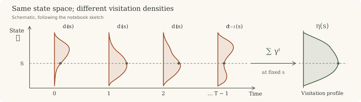
Note $S_t$ takes values in the same state space $\mathcal S$, and $A_t$ in the same action space $\mathcal A$, so when we integrate over $s_t$ and $a_t$ it means integrating over $\mathcal S$ and $\mathcal A$ ($s_t$ and $a_t$ are dummy vars). Schematics below shows intuition on how we can transition from summing over time and then integrating to marginalizing across time steps.

Let $d_t^{\pi_\theta}(s)$ denote the marginal density of $S_t$ at $s$ (for discrete states, $d_t^{\pi_\theta}(s)=\Pr(S_t=s)$). The time step is part of the function $d_t^{\pi_\theta}$, not of its argument: the same state $s$ generally has a different density at each time step. If we define:

$$\eta_\gamma^{\pi_\theta}(s):=\sum_{t=0}^{T-1}\gamma^t d_t^{\pi_\theta}(s).$$

The best way to look at it to get intuition is that for $\gamma=1$ and discrete case it is just expected number of visits to a state $s \in \mathcal S$.

Next:

In this post we derived foundations of policy gradient methods and in the next post we will try to map the concepts we learned here (in a more classical RL setting) into RL for LLMs.

¹ These are sufficient conditions chosen to keep the derivation simple, rather than necessary conditions. ↩

² Sutton and Barto write $\mathbb E_{\pi_\theta}$ for expectation when following policy $\pi_\theta$ in the environment. The policy, environment dynamics, and initial-state distribution together induce our trajectory distribution $p_\theta(\tau)$. Thus $\mathbb E_{p_\theta(\tau)}[G_t\mid S_t=s,A_t=a]$ and $\mathbb E_{\pi_\theta}[G_t\mid S_t=s,A_t=a]$ denote the same conditional expectation, including both policy and environment randomness. See Chapter 3. ↩

³ In our fixed-horizon episodic setting, this notation implicitly includes the time step in the state. The same underlying state-action pair can have different values depending on how many steps remain before the terminal time $T$. Including time in the state lets us write $Q_{\pi_\theta}(s,a)$ without a separate time index. ↩

⁴ Including the time step in the state makes these results applicable to fixed-horizon problems. However, visits to the same underlying state at different times now count as visits to different augmented states. The visitation formulation remains valid, but it no longer combines those visits into a single weight for the underlying state. ↩

References and further reading

• Richard S. Sutton and Andrew G. Barto. Reinforcement Learning: An Introduction, second edition, Chapters 3 and 13.
• Ronald J. Williams. Simple Statistical Gradient-Following Algorithms for Connectionist Reinforcement Learning, 1992.
• OpenAI Spinning Up. Introduction to Policy Optimization.
• Qingfeng Lan. From REINFORCE to Dr. GRPO - really great read and tbh one of inspirations for this series!