Data Efficiency of RL Prediction Methods in Environments with Terminal-Only Rewards

Learning from limited experience

In this post we will explore how sample-efficient different prediction methods are in RL environments with only terminal rewards. More specifically, we will visualize the mechanisms that can affect sample efficiency in these environments. Why is this interesting? Many complex, long-term tasks combine two difficulties: collecting a trajectory is expensive (so we need sample-efficient learning) and assigning rewards to intermediate steps is difficult, while judging the final outcome is more straightforward.

Before going any further let's just clearly define what sample efficiency is: Sample efficiency is how much experience (measured in transitions or episodes) a method needs to reach a given level of prediction accuracy. We will examine two aspects of how prediction methods (for simplicity we are looking at tabular methods here) use experience in this setting and how each of these aspects is used in different prediction algorithms:

1. Learning from a single episode - once the terminal reward is observed, how far back does that information propagate along the trajectory and how strongly does it affect value function estimates of intermediate states in the trajectory?
2. Learning across episodes - how do we leverage information learned in one episode to improve value estimates across trajectories in the other episode?

A bit more intuition about learning across episodes

One interesting and very visually appealing way of thinking about how different tabular RL prediction algorithms leverage experience across multiple episodes is thinking in terms of intersections between trajectories (this analogy is really well illustrated by exercise 6.2 in Sutton and Barto's book). Intersections of trajectories act as conduits through which information between episodes is propagated and learnt. Conceptually, how we utilize these shared states between trajectories answers the question of how we leverage information from one episode to learn faster in another one.
In many dense reward environments, where many intermediate transitions provide reward, most of the bootstrapping methods can leverage intersections without waiting for the trajectory to end; however, in environments with terminal-only rewards, the depth of the backup operator plays a key role, because in order for shared states between trajectories to be leveraged, information needs to be propagated to those states (note how strongly that backup operator influences that state’s value estimate matters as well!).

In this post, I want to go through several popular RL algorithms with visualizations and follow the updates on the same three trajectories to illustrate the difference in how shared states are utilized, but before that let's quickly cover a simple environment which we will be using for demonstration.

The environment

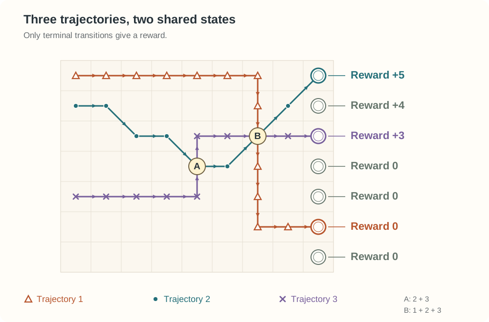
Let us consider a simple grid environment where all intermediate rewards are zero. An episode ends when we reach the right edge, with rewards of 5, 4, 3, 0, 0, 0, and 0 from top to bottom. We will follow three trajectories observed under a fixed policy, ending with rewards of 0, +5, and +3. They share two states: A, visited by trajectories 2 and 3, and B, visited by all three. We initialize state values to zero and set $\gamma = 1$ to keep the example simple. With no intermediate rewards or step costs, trajectories ending with the same reward have the same return regardless of their length. In a control problem, this would give the agent no incentive to prefer a shorter route to the same positive reward. Here, we are evaluating a fixed policy rather than choosing actions, so using undiscounted rewards doesn't lead to bad outcomes, but simplifies the example from the perspective of illustration.

In the grid I sketched, the trajectories end at different terminal states. There are two intersection points that I want to focus on:

• Point A is shared by trajectories 2 and 3.
• Point B is shared by all three trajectories.

Following the updates

Let us now go through the methods one by one and follow how they use the same three trajectories. For MC, we average the observed returns with a step size of $\frac{1}{N(s)}$. For the TD methods, we start with $\alpha = 1$ so that each update is easy to follow. These are illustrations of how information is used; a larger change in a value estimate does not by itself mean that we learned a more accurate value.

Monte Carlo

Let us start with the most straightforward approach - MC. After an episode ends, we update each visited state using the return observed from that state:

$$V(S_t) \leftarrow V(S_t) + \frac{1}{N(S_t)}\bigl[G_t - V(S_t)\bigr]$$

Here $N(s)$ counts the returns averaged at state s, including the current one.¹ With $\gamma = 1$ and no intermediate rewards, the return from every nonterminal state on a trajectory is simply its terminal reward.

MC combines returns from different episodes at shared states, but it does not use their updated estimates to revise values along other trajectories. Learning across episodes is therefore limited to the intersections themselves. Within each episode, however, MC uses the terminal outcome to update every visited nonterminal state.

TD(0)

With TD(0), we do not need to wait until the episode ends. After each transition, we update the state we just left using the observed reward and the discounted estimate of the next state's value:

$$V(S_t) \leftarrow V(S_t) + \alpha\bigl[R_{t+1} + \gamma V(S_{t+1}) - V(S_t)\bigr]$$

Theoretically, this allows us to use shared states between trajectories: if the next state is an intersection whose value is already informative (from a previous episode's update), that state's value function estimate can be leveraged on the current trajectory. TD essentially leverages the Markov assumption - the state's expected future return under our fixed policy does not depend on which path brought us there.

The difficulty in our sparse-reward example environment is that the TD(0) backup operator has a low depth of update, so if intersections are far away from the terminal state, the update will not reach them - and hence intersections between trajectories are not leveraged at all! In our visualization, terminal reward information does not even reach B, the intersection closest to the terminal states. So while theoretically TD(0) leverages shared states, in sparse reward situations insufficient depth of update might mean it is unable to do so.

As we observe more trajectories, some will intersect states whose values already were updated by the TD(0) backup operator. TD(0) can then use those value function estimates to carry information one transition further back along the new trajectory. Over successive episodes, information can gradually spread through these shared states. However, without replay, we do not return to earlier trajectories to revise their estimates using what we learned later. Their stored transitions could connect earlier states to newly created intersections, but those connections are not used again unless we replay them.

So, although bootstrapping allows TD(0) to learn across trajectories, its one-step backups and lack of replay can delay the spread of terminal reward information. Transitions in earlier episodes may be processed before their successor states have informative estimates, and without replay we cannot reuse those particular observations once better estimates become available.

n-step TD

With n-step TD, an update can use rewards observed over a longer part of the trajectory before bootstrapping. For states within $n$ transitions of the terminal state, the target is simply the sum of discounted rewards up to termination, with no bootstrap. Notice that this is the same target as MC (the update rule, though, is different because of the learning rate).

$$G_t^{(n)} = \begin{cases} \displaystyle\sum_{k=1}^{n}\gamma^{k-1}R_{t+k} + \gamma^n V(S_{t+n}), & t+n < T, \\[6pt] \displaystyle\sum_{k=1}^{T-t}\gamma^{k-1}R_{t+k} = G_t, & t+n \ge T. \end{cases}$$

$$V(S_t) \leftarrow V(S_t) + \alpha\bigl[G_t^{(n)} - V(S_t)\bigr]$$

Here $T$ is the time at which the episode terminates, so $T-t$ is the number of transitions remaining from $S_t$. If termination occurs within the next $n$ transitions, we use the rewards up to termination and omit the bootstrap - essentially it then becomes equivalent to the MC update.

Try comparing 3- and 5-step TD backups in the visualization: with 3-step TD, by the time trajectory 3 reaches intersection B, the value function for that state has already been updated and we propagate information through the TD(3) backup without waiting until the terminal state. In TD(3), the backup operator is too shallow to reach intersection A in trajectory 2 so that it can be leveraged in the trajectory 3 backup; however, if you play TD(5) in the visualization tool, you can see clearly that intersection A is also leveraged to transfer experience from the 2nd trajectory to the 3rd trajectory. Notice how the number of states reached by nonzero reward information and the ability to leverage past experience increased with the depth of the backup operator from TD(0) to TD(3) and TD(5). So n-step TD can have a sufficiently deep backup operator to propagate terminal reward deeper into the trajectory's intermediate states and can leverage intersections to learn across trajectories through bootstrapping. Together, these mechanisms can help n-step TD learn more efficiently than TD(0) in environments with only terminal rewards.

A couple of interesting drawbacks to notice in n-step TD:

1. Like any online learning algorithm, it still does not revisit states unique to earlier trajectories. Their estimates remain unchanged unless we visit them again or reuse their stored experience. Increasing backup depth does not by itself resolve this limitation.
2. n-step TD bootstraps only from the value estimate exactly n steps ahead, unless the episode terminates sooner. This means that even if some intermediate states already have informative estimates, the current update does not directly benefit from them. In our sparse-reward example, if the n-step window along the trajectory contains no terminal reward and the bootstrap state still has value zero, the target remains zero, even when states between the current state and the bootstrap state have already learned something. An interesting insight here is that it is not only the depth of the backup operator that is important, but exactly which learned estimates it uses. In our example, we can see this in the TD(5) visualization: some states remain at zero even though states farther back along the same trajectory have already received nonzero updates. Each update depends on the estimate exactly five steps ahead, so informative estimates in between are not directly used.

TD(λ)

For the purpose of this blog, let us start with the forward view of TD(λ).² With n-step TD, we choose a particular depth for the backup. TD(λ) instead combines returns from different backup depths, with $\lambda$ controlling their weights.

$$G_t^\lambda = (1-\lambda)\sum_{n=1}^{T-t-1}\lambda^{n-1}G_t^{(n)} + \lambda^{T-t-1}G_t$$

Here $G_t^{(n)}$ is the n-step return from the previous section, $G_t$ is the full return, and $T$ is the time at which the episode ends. The last term collects the remaining weight at the terminal outcome. Since TD(λ) combines returns from different backup depths, allowing estimates at multiple points along the trajectory to contribute, each $G_t^{n}$ will contain bootstrapping from the value estimate n steps ahead; the important implication of this is that TD(λ), in comparison to n-step TD, would not miss informative value estimates at intermediate states.
Once the episode is complete, we can use this weighted return as our update target:

$$V(S_t) \leftarrow V(S_t) + \alpha\bigl[G_t^\lambda - V(S_t)\bigr]$$

In some ways, we can think of this as an expectation over backup depths, where the backup depth is distributed as a geometric random variable. After each transition, with probability $1-\lambda$ we decide to stop the backup and bootstrap from the current state's value, or with probability $\lambda$ we continue one transition further. If we reach the terminal state, we stop with the full observed return and no bootstrap.
The most important point for this post is that TD(λ) combines two useful properties. First, terminal reward information can propagate through the full depth of a trajectory, potentially reaching intersections that a shorter backup would miss. Second, it combines returns that bootstrap from intermediate states at different distances, rather than only from the state exactly n steps ahead (like n-step TD does). This allows it to use a broader set of intersections and the information accumulated at them across previous episodes.
In this sense, TD(λ) combines the reach of MC with TD’s ability to reuse learned value estimates. However, there is no free lunch: reaching a state does not mean updating it strongly. λ controls the balance. A smaller λ puts more weight on short bootstrapped returns, while the influence of the terminal outcome fades more quickly with distance. A larger λ gives more weight to longer returns, but less to intermediate bootstrap estimates - this is easy to see at the extremes: at λ = 0, the target reduces to the TD(0) target $G_t^{(1)}$; at λ = 1, it becomes the full MC return $G_t$.

If you play the visualization, you can see how information from previous episodes propagates back along the current trajectory, with both intersections used to share information between trajectories. Notice that with TD(5), some states remain at zero even though states farther back along the same trajectory have already received nonzero updates. TD(λ) fills in these gaps in our example because, as I mentioned earlier, it combines multiple backup depths rather than relying on a single n-step bootstrap. However, we still do not revisit the states in the first trajectory before intersection B. These states remain at zero even after later episodes provide information that replay could propagate to them.

Batch TD(0)

TD(λ) can carry information farther along the current trajectory, but it still leaves states unique to earlier trajectories unchanged. Batch TD addresses this by revisiting stored transitions and updating earlier paths using information learned later.

Batch TD repeatedly applies TD(0) backups to the stored experience, updating all observed nonterminal states in parallel in our implementation. Interestingly, just a little algebra shows that its fixed point is the value function of the maximum-likelihood MRP estimated from trajectories collected under our fixed policy.

$$v(s) \leftarrow v(s) + \frac{\alpha}{N(s)}\sum_i\sum_{t:\,S_t^{(i)}=s}\bigl[R_{t+1}^{(i)} + \gamma v(S_{t+1}^{(i)}) - v(s)\bigr]$$

Every target in a sweep uses the values from the previous sweep, so newly learned information moves one transition backward per sweep, and that happens across all trajectories. So not only do later trajectories leverage intersections, but earlier ones do as well.

In the visualization, we first collect all three episodes and then make repeated passes, or sweeps, through the stored transitions. For each visited nonterminal state, we average its TD errors.

Notice what happens at B. Once information from the three observed continuations reaches it, its estimate becomes $V(B) = (0 + 5 + 3)/3 = 8/3$. Subsequent sweeps carry that estimate backward along the stored paths leading to B, including trajectory 1. Even though that episode ended with reward zero, its states before B can now use information from the other two episodes. MC keeps those states at zero in this example, while batch TD eventually gives them a value of $8/3$.

This is the kind of sharing through intersections that we could not get by making just one pass through the earlier trajectories. The backup still has a depth of one, but repeated sweeps let information travel farther and reach states we have not visited again.

Experiments

Batch MC vs. Batch TD

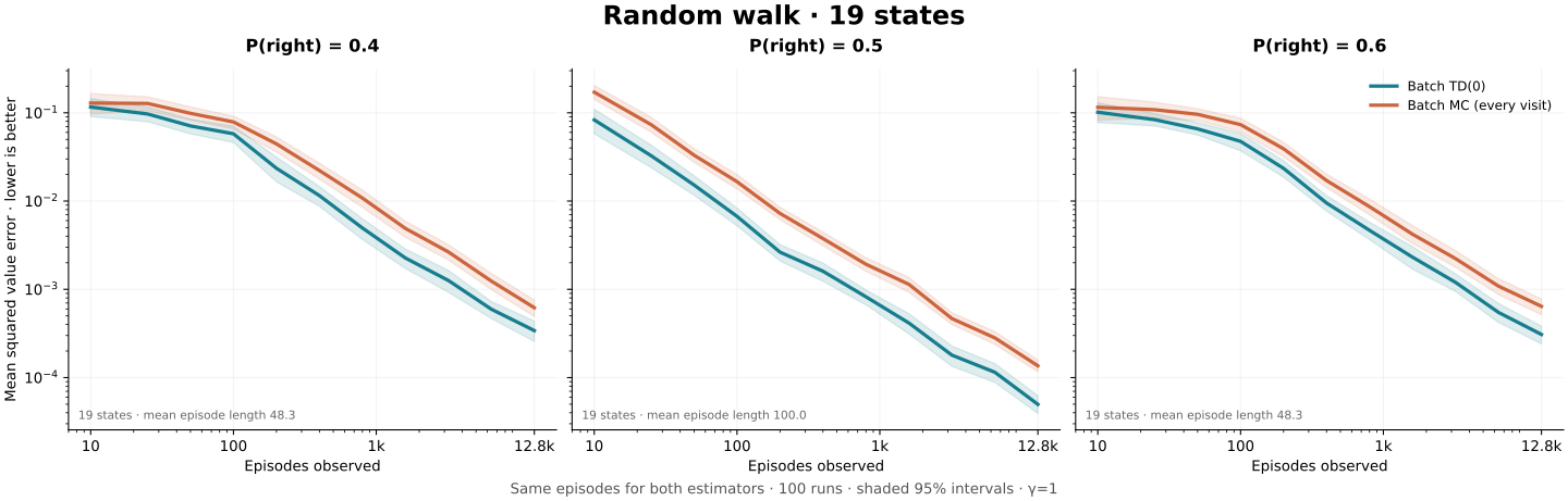
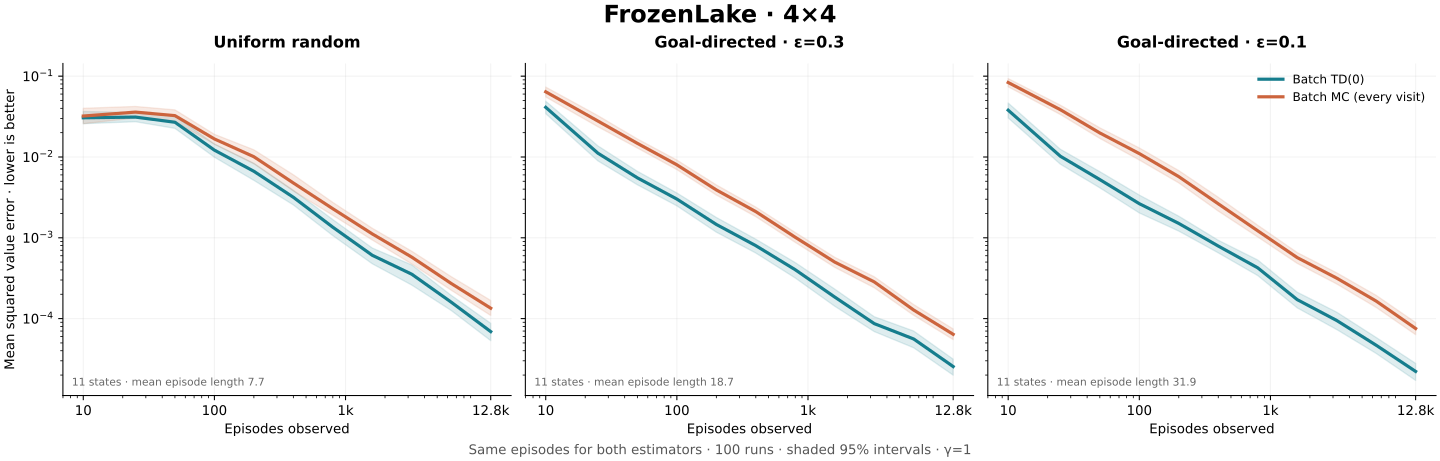
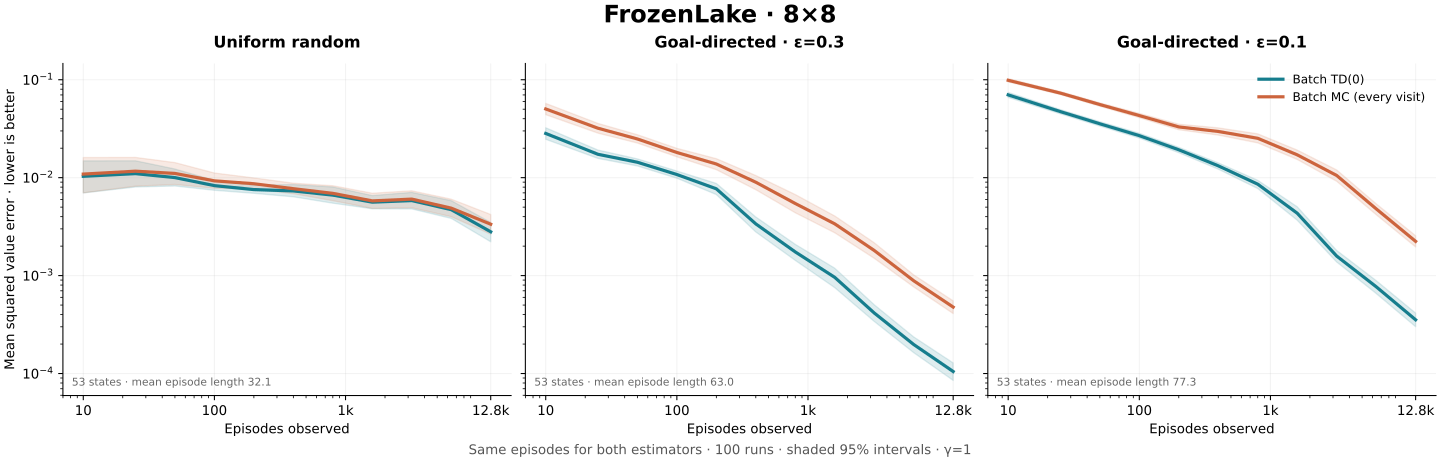
Batch MC averages observed returns at each state. Batch TD also uses intersections to carry information between trajectories, including earlier ones. This gives us a reason to expect better sample efficiency when trajectories share states: experience collected on one path can improve estimates on another.

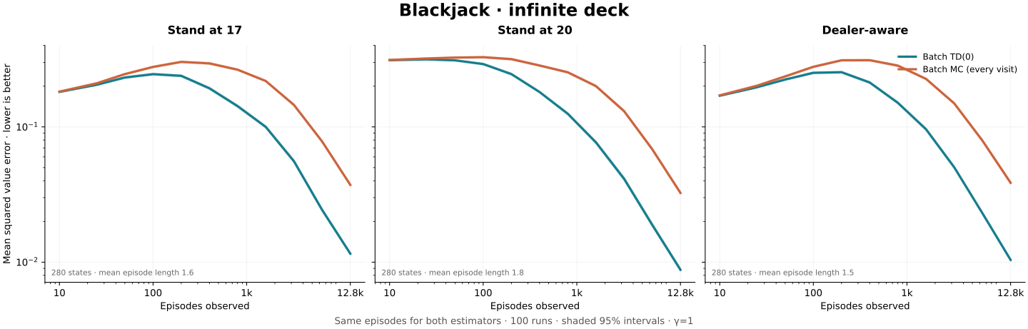
To test this expectation, we compared the methods on a 19-state random walk, FrozenLake (4×4 and 8×8), and Blackjack, with three fixed policies each and 100 independent runs. Both methods received identical episodes. We measured MSE against exact policy values across all reachable nonterminal states.

At 3,200 episodes, Batch TD had lower mean MSE in all 12 settings: MC’s error was roughly 1.9–3.2 times larger on random walk and Blackjack, and up to 6.7 times larger on FrozenLake. Note that these results, while aligned with our expectation, by themselves don't prove that intersections and the way batch TD utilizes them through bootstrapping are the cause of batch TD's outperformance.
One other thing to mention is that technically batch TD usually would cost more computation.

How much does sharing through intersections help?

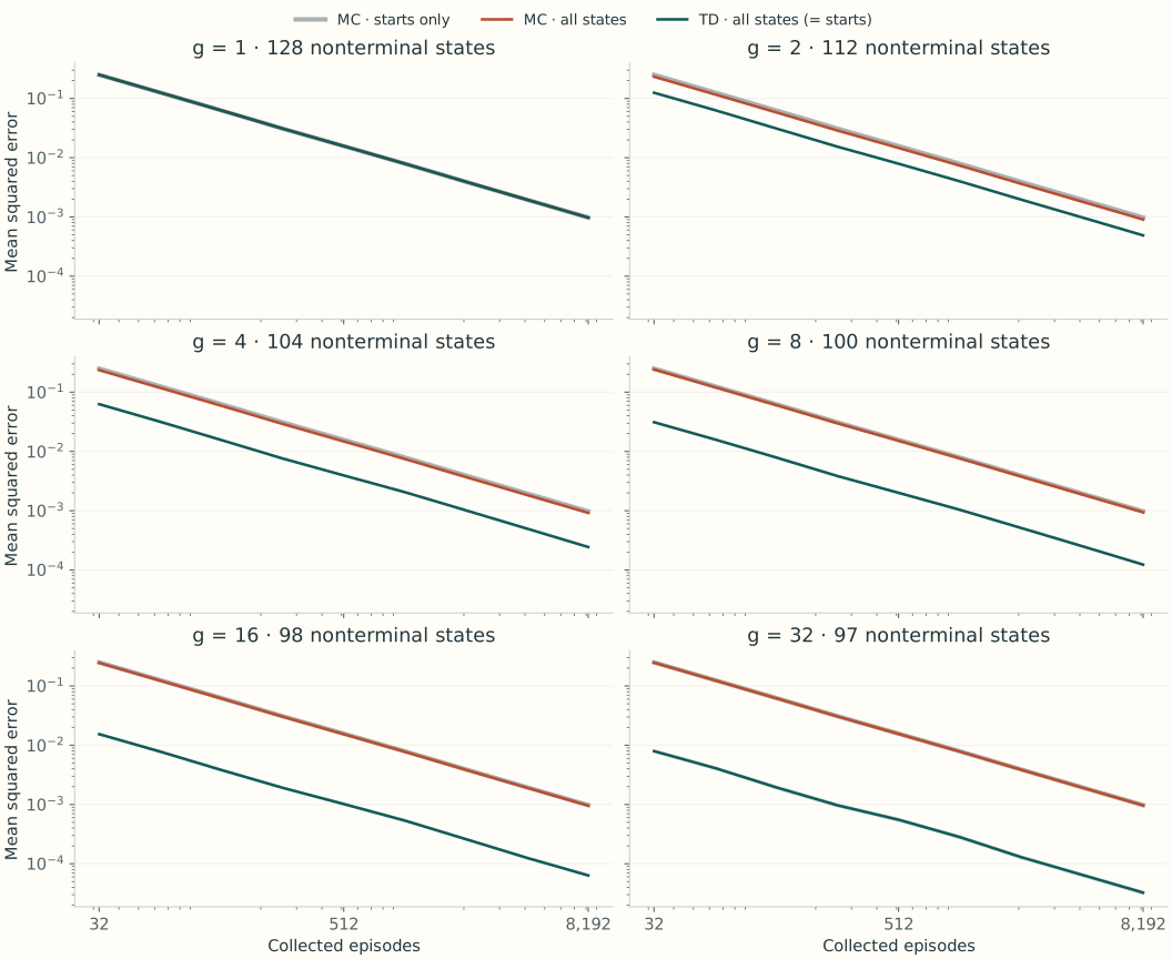
Let's try to create an experiment that isolates the effect of sharing between trajectories. We use 32 starting states, each with two private intermediate states before reaching a downstream state. We vary how many starting paths share that state: $g=1,2,4,8,16,32$. Every episode takes four transitions and ends with a reward of 0 or 1, each with probability $0.5$. All transitions until the terminal state transition have a reward of $0$.

Each row starts with a private path. Change $g$ to see how many paths merge into the same downstream state; the highlighted group shares $H_1$. Episode length and reward distribution stay unchanged.

We collect equally many episodes from each starting state. Both methods receive the same data (i.e. the same trajectories), and when we change how paths merge, we keep each episode’s terminal reward unchanged. This helps us to isolate the effect of information sharing through intersections.

With no sharing between different starts ($g=1$), Batch MC and Batch TD give identical estimates. As sharing increases (i.e. $g$ increases), batch TD becomes more accurate. At 1,024 episodes, MC’s all-state MSE is about 1.8 times larger than TD’s for $g=2$, 7.4 times larger for $g=8$, and 27.8 times larger for $g=32$ - this is the result you would expect!

The explanation is simple: with $m$ episodes per start, MC averages $m$ returns at each private state and $gm$ returns at states closer to the terminal state. Batch TD also pools those $gm$ outcomes, but carries the resulting estimate back to each private path. It is essentially using shared states to transfer information between private entry paths. This idea is also easy to visualize by looking at the heatmap of MSEs per state - where we observe virtually no difference between MC and batch TD in shared states and the absolute majority of the difference coming from private paths.

Conclusion

Looking mechanistically at how each prediction method learns from trajectories in a terminal-only reward environment suggests that sample efficiency in this setting depends on three questions:

1. How deep is the backup operator? A terminal reward can only improve a state's estimate once it has propagated back to that state. And bootstrapping methods can be effective only if trajectory reaches intersections. TD(0) moves it one transition per update, n-step TD moves it n transitions. MC and TD(λ) can reach the whole trajectory, though TD(λ)'s effective depth depends on $\lambda$, meaning that with low values of lambda terminal reward would essentially be heavily discounted (even with $\gamma=1$) and its contribution will fade quickly with distance from terminal state. Batch TD can also go full depth because of repeated updates.
2. Which learned estimates does the update use? Reaching an intersection does not mean an update uses the value estimate learned there. An n-step TD update bootstraps only from the state exactly n steps ahead; it does not bootstrap using value estimates of intersections before that n-step endpoint. TD(λ) in contrast will utilize existing values estimate of any intersection that is on the path of trajectory.
3. Do we go back to earlier trajectories? Online methods only improve the path they are currently on. Batch TD revisits stored transitions, so what we learn at an intersection later flows back to paths we observed earlier.

References

• Richard S. Sutton and Andrew G. Barto. Reinforcement Learning: An Introduction, second edition, 2018. Chapters 5, 6, 7, and 12 cover Monte Carlo, TD, n-step methods, and TD(λ).
• Sam Greydanus and Chris Olah. The Paths Perspective on Value Learning, Distill, 2019. I found this article after writing this post. It develops very closely related ideas about how TD learning combines experience at intersections between trajectories.